Penn World Table 9.1 in R
Fred Viole
10/8/2019
1 Intro
The objective of this analysis is to try to capture any causative effects in the Penn World Table data on Real GDP rdgpe.
We will use several techniques available on a theoretical ground truth,
and then apply the most accurate technique on the remaining variables.
1.1 Ground Truth
The ground truth we have identified is that Real GDP causes Total Factor Productivity tfp. Why is this? The contention is that tfp
is essentially measuring economies of scale, and in order to invoke
those economies of scale, a country must first achieve scale! Thus, we
assume rdgpe causes tfp.
2 PWT 9.1 Data
- Download the pwt91.xlsx file by clicking here.
- Select the
Datasheet and save it as a.csvfile. - Move the
.csvfile to your working R directory, then load into R as adata.table.
library(data.table)

pwt <- fread("pwt91.csv", header = TRUE)
3 Select Relevant Subgroups and Variable of Interest
To select individual countries, simply create a vector of interested countries using the countrycode or coutry variable and create a new data.table.
The dependent variable of interest is rgdpe measures.
3.1 Variable Legend
| Identifier variables | . . |
| countrycode | 3-letter ISO country code . . |
| country | Country name . . |
| currency_unit | Currency unit . . |
| year | Year . . |
| . . | |
| Real GDP, employment and population levels | . . |
| rgdpe | Expenditure-side real GDP at chained PPPs (in mil. 2011US$) . . |
| rgdpo | Output-side real GDP at chained PPPs (in mil. 2011US$) . . |
| pop | Population (in millions) . . |
| emp | Number of persons engaged (in millions) . . |
| avh | Average annual hours worked by persons engaged . . |
| hc | Human capital index, based on years of schooling and returns to education; see Human capital in PWT9. . . |
| . . | |
| Current price GDP, capital and TFP | . . |
| ccon | Real consumption of households and government, at current PPPs (in mil. 2011US$) . . |
| cda | Real domestic absorption, (real consumption plus investment), at current PPPs (in mil. 2011US$) . . |
| cgdpe | Expenditure-side real GDP at current PPPs (in mil. 2011US$) . . |
| cgdpo | Output-side real GDP at current PPPs (in mil. 2011US$) . . |
| cn | Capital stock at current PPPs (in mil. 2011US$) . . |
| ck | Capital services levels at current PPPs (USA=1) . . |
| ctfp | TFP level at current PPPs (USA=1) . . |
| cwtfp | Welfare-relevant TFP levels at current PPPs (USA=1) . . |
| . . | |
| National accounts-based variables | . . |
| rgdpna | Real GDP at constant 2011 national prices (in mil. 2011US$) . . |
| rconna | Real consumption at constant 2011 national prices (in mil. 2011US$) . . |
| rdana | Real domestic absorption at constant 2011 national prices (in mil. 2011US$) . . |
| rnna | Capital stock at constant 2011 national prices (in mil. 2011US$) . . |
| rkna | Capital services at constant 2011 national prices (2011=1) . . |
| rtfpna | TFP at constant national prices (2011=1) . . |
| rwtfpna | Welfare-relevant TFP at constant national prices (2011=1) . . |
| labsh | Share of labour compensation in GDP at current national prices . . |
| irr | Real internal rate of return . . |
| delta | Average depreciation rate of the capital stock . . |
| . . | |
| Exchange rates and GDP price levels | . . |
| xr | Exchange rate, national currency/USD (market+estimated) . . |
| pl_con | Price level of CCON (PPP/XR), price level of USA GDPo in 2011=1 . . |
| pl_da | Price level of CDA (PPP/XR), price level of USA GDPo in 2011=1 . . |
| pl_gdpo | Price level of CGDPo (PPP/XR), price level of USA GDPo in 2011=1 . . |
| . . | |
| Data information variables | . . |
| i_cig | 0/1/2: relative price data for consumption, investment and government is extrapolated (0), benchmark (1) or interpolated (2) . . |
| i_xm | 0/1/2: relative price data for exports and imports is extrapolated (0), benchmark (1) or interpolated (2) . . |
| i_xr | 0/1: the exchange rate is market-based (0) or estimated (1) . . |
| i_outlier | 0/1: the observation on pl_gdpe or pl_gdpo is not an outlier (0) or an outlier (1) . . |
| i_irr | 0/1/2/3: the observation for irr is not an outlier (0), may be biased due to a low capital share (1), hit the lower bound of 1 percent (2), or is an outlier (3) . . |
| cor_exp | Correlation between expenditure shares of the country and the US (benchmark observations only) . . |
| statcap | Statistical capacity indicator (source: World Bank, developing countries only) . . |
| . . | |
| Shares in CGDPo | . . |
| csh_c | Share of household consumption at current PPPs . . |
| csh_i | Share of gross capital formation at current PPPs . . |
| csh_g | Share of government consumption at current PPPs . . |
| csh_x | Share of merchandise exports at current PPPs . . |
| csh_m | Share of merchandise imports at current PPPs . . |
| csh_r | Share of residual trade and GDP statistical discrepancy at current PPPs . . |
| . . | |
| Price levels, expenditure categories and capital | . . |
| pl_c | Price level of household consumption, price level of USA GDPo in 2011=1 . . |
| pl_i | Price level of capital formation, price level of USA GDPo in 2011=1 . . |
| pl_g | Price level of government consumption, price level of USA GDPo in 2011=1 . . |
| pl_x | Price level of exports, price level of USA GDPo in 2011=1 . . |
| pl_m | Price level of imports, price level of USA GDPo in 2011=1 . . |
| pl_n | Price level of the capital stock, price level of USA in 2011=1 . . |
| pl_k | Price level of the capital services, price level of USA=1 . . |
3.2 Selecting Countries by coutnry or countrycode
Just an example for various subsetting…
countries <- c("China", "Singapore", "Taiwan", "Viet Nam", "Myanmar", "Thailand",
               "Japan", "South Africa", "Bangladesh", "India", "Indonesia")

pwt_subset <- pwt[pwt$country%in%countries | pwt$countrycode%in%countries,]

require(ggplot2)
ggplot(pwt_subset, aes(x = year, y = rgdpe, col = country)) + geom_line()
3.3 Step 1: Select only Countries with pop > 1mm
The first year of US data is 1954, so we need to eliminate the other years, and only select countries with 1mm people or more.
pwt_1 <- pwt[pop > 1 & year >= 1954,]3.4 Step 2: Find the Countries with No ctfp Data
ctfp_countries <- pwt_1[, sum(is.na(ctfp))/.N, by=country]
full_ctfp_countries <- ctfp_countries[V1==0, country]

pwt_2 <- pwt_1[country%in%full_ctfp_countries,]
3.5 Step 3: NNS Causation Method
library(NNS)
NNS_Caus <- pwt_2[, NNS_Causation_Direction := names(NNS.caus(rgdpe, ctfp, tau = 3)[3]), by=country]

NNS_Caus <- pwt_2[, NNS_Causation := as.numeric(NNS.caus(rgdpe, ctfp,tau = 3)[3]), by=country]

NNS_Caus[,unique(.SD),.SDcols=c("NNS_Causation","NNS_Causation_Direction"), by=country]| country<chr> | NNS_Causation<dbl> | NNS_Causation_Direction<chr> |
|---|---|---|
| Argentina | 0.65766672 | C(x—>y) |
| Australia | 0.01633652 | C(x—>y) |
| Austria | 0.00000000 | C(x—>y) |
| Belgium | 0.41123278 | C(x—>y) |
| Bahrain | 0.00000000 | C(x—>y) |
| Bolivia (Plurinational State of) | 0.41297688 | C(x—>y) |
| Brazil | 0.31770500 | C(x—>y) |
| Botswana | 0.54041620 | C(x—>y) |
| Canada | 0.64213690 | C(x—>y) |
| Switzerland | 0.32310106 | C(x—>y) |
1-10 of 51 rows
3.5.1 NNS: Countries NOT to show rdgpe causes ctfp
NNS_Caus[NNS_Causation_Direction=="C(y--->x)", unique(country)]## [1] "Eswatini"3.6 Step 4: Granger Causality
library(lmtest)
granger <- pwt_2[countrycode!="USA",]

granger <- granger[, granger_causality := grangertest(ctfp ~ rgdpe, order=3)$Pr[2], by=country]
3.6.1 Granger: Countries NOT to show rdgpe causes ctfp
granger[granger_causality > 0.05, unique(country)]## [1] "Australia" "Austria"
## [3] "Belgium" "Bahrain"
## [5] "Bolivia (Plurinational State of)" "Brazil"
## [7] "Switzerland" "Colombia"
## [9] "Costa Rica" "Germany"
## [11] "Denmark" "Ecuador"
## [13] "Egypt" "Spain"
## [15] "Finland" "France"
## [17] "Gabon" "United Kingdom"
## [19] "Guatemala" "Ireland"
## [21] "Israel" "Italy"
## [23] "Jordan" "Japan"
## [25] "Kenya" "Kuwait"
## [27] "Sri Lanka" "Morocco"
## [29] "Mexico" "Mauritius"
## [31] "Namibia" "Netherlands"
## [33] "Norway" "New Zealand"
## [35] "Peru" "Philippines"
## [37] "Portugal" "Qatar"
## [39] "Sweden" "Thailand"
## [41] "Trinidad and Tobago" "Turkey"
## [43] "Uruguay"3.7 Step 5: generalCorr Causality
library(generalCorr)

gc <- pwt_2[countrycode!="USA",]
gc <- gc[, gc_causality := causeSummBlk(cbind(ctfp, rgdpe))[1], by=country]
## [1] ctfp causes rgdpe strength= 100
## [1] corr= 0.8279 p-val= 0
## [1] ctfp causes rgdpe strength= 31.496
## [1] corr= 0.2329 p-val= 0.06405
## [1] rgdpe causes ctfp strength= -37.008
## [1] corr= 0.4776 p-val= 7e-05
## [1] rgdpe causes ctfp strength= -37.008
## [1] corr= 0.4622 p-val= 0.00012
## [1] rgdpe causes ctfp strength= -100
## [1] corr= -0.1893 p-val= 0.5773
## [1] ctfp causes rgdpe strength= 100
## [1] corr= -0.3249 p-val= 0.00881
## [1] rgdpe causes ctfp strength= -37.008
## [1] corr= -0.1903 p-val= 0.13202
## [1] rgdpe causes ctfp strength= -37.008
## [1] corr= -0.7775 p-val= 0
## [1] rgdpe causes ctfp strength= -37.008
## [1] corr= -0.7161 p-val= 0
## [1] rgdpe causes ctfp strength= -37.008
## [1] corr= 0.3954 p-val= 0.00122
## [1] rgdpe causes ctfp strength= -37.008
## [1] corr= -0.033 p-val= 0.79558
## [1] rgdpe causes ctfp strength= -37.008
## [1] corr= -0.8033 p-val= 0
## [1] rgdpe causes ctfp strength= -100
## [1] corr= 0.9408 p-val= 0
## [1] rgdpe causes ctfp strength= -37.008
## [1] corr= 0.7007 p-val= 0
## [1] ctfp causes rgdpe strength= 15.748
## [1] corr= -0.6441 p-val= 0
## [1] rgdpe causes ctfp strength= -37.008
## [1] corr= 0.0382 p-val= 0.76471
## [1] rgdpe causes ctfp strength= -37.008
## [1] corr= 0.2844 p-val= 0.02275
## [1] rgdpe causes ctfp strength= -37.008
## [1] corr= 0.8128 p-val= 0
## [1] rgdpe causes ctfp strength= -0.787
## [1] corr= 0.5687 p-val= 0
## [1] rgdpe causes ctfp strength= -37.008
## [1] corr= -0.5455 p-val= 0.00395
## [1] rgdpe causes ctfp strength= -37.008
## [1] corr= 0.4811 p-val= 6e-05
## [1] ctfp causes rgdpe strength= 37.008
## [1] corr= -0.8594 p-val= 0
## [1] rgdpe causes ctfp strength= -37.008
## [1] corr= 0.8916 p-val= 0
## [1] ctfp causes rgdpe strength= 100
## [1] corr= 0.7794 p-val= 0
## [1] rgdpe causes ctfp strength= -100
## [1] corr= 0.4512 p-val= 0.00018
## [1] ctfp causes rgdpe strength= 48.819
## [1] corr= 0.3048 p-val= 0.01433
## [1] rgdpe causes ctfp strength= -37.008
## [1] corr= -0.3862 p-val= 0.003
## [1] rgdpe causes ctfp strength= -100
## [1] corr= 0.8525 p-val= 0
## [1] rgdpe causes ctfp strength= -100
## [1] corr= -0.6594 p-val= 0
## [1] ctfp causes rgdpe strength= 100
## [1] corr= -0.0035 p-val= 0.98227
## [1] ctfp causes rgdpe strength= 50.394
## [1] corr= -0.0243 p-val= 0.84901
## [1] rgdpe causes ctfp strength= -37.008
## [1] corr= -0.7686 p-val= 0
## [1] rgdpe causes ctfp strength= -37.008
## [1] corr= -0.8332 p-val= 0
## [1] rgdpe causes ctfp strength= -100
## [1] corr= -0.8619 p-val= 0
## [1] rgdpe causes ctfp strength= -100
## [1] corr= -0.5249 p-val= 0.00072
## [1] ctfp causes rgdpe strength= 100
## [1] corr= 0.4172 p-val= 6e-04
## [1] rgdpe causes ctfp strength= -37.008
## [1] corr= 0.8874 p-val= 0
## [1] rgdpe causes ctfp strength= -37.008
## [1] corr= 0.3136 p-val= 0.01164
## [1] rgdpe causes ctfp strength= -37.008
## [1] corr= -0.3469 p-val= 0.00499
## [1] rgdpe causes ctfp strength= -37.008
## [1] corr= -0.1066 p-val= 0.40176
## [1] rgdpe causes ctfp strength= -37.008
## [1] corr= -0.4865 p-val= 5e-05
## [1] rgdpe causes ctfp strength= -100
## [1] corr= -0.3775 p-val= 0.22638
## [1] rgdpe causes ctfp strength= -37.008
## [1] corr= 0.3768 p-val= 0.00215
## [1] rgdpe causes ctfp strength= -37.008
## [1] corr= -0.8835 p-val= 0
## [1] rgdpe causes ctfp strength= -37.008
## [1] corr= 0.148 p-val= 0.2433
## [1] ctfp causes rgdpe strength= 37.008
## [1] corr= -0.084 p-val= 0.59208
## [1] rgdpe causes ctfp strength= -100
## [1] corr= 0.7847 p-val= 0
## [1] ctfp causes rgdpe strength= 100
## [1] corr= -0.5156 p-val= 1e-05
## [1] rgdpe causes ctfp strength= -100
## [1] corr= -0.5238 p-val= 1e-05
## [1] rgdpe causes ctfp strength= -37.008
## [1] corr= -0.6665 p-val= 03.7.1 generalCorr: Countries NOT to show rdgpe causes ctfp
gc[gc_causality=="ctfp", unique(country)]## [1] "Argentina" "Australia"
## [3] "Bolivia (Plurinational State of)" "Ecuador"
## [5] "Guatemala" "Ireland"
## [7] "Italy" "Kuwait"
## [9] "Sri Lanka" "Netherlands"
## [11] "Trinidad and Tobago" "Uruguay"So if theoretically rgdpe causes ctfp, and 2 of the state of the art methodologies agree, then what causes rdgpe???
4 Finding Other Causative Variables
Reviewing the literature may offer some ability to narrow down this search based on economic theory.
4.1 Hall and Jones (1999)
Output per worker varies enormously across countries. Why? On an accounting basis our analysis shows that differences in physical capital and educational attainment can only partially explain the variation in output per worker. They find a large amount of variation in the level of the Solow residual across countries. At a deeper level, we document that the differences in capital accumulation, productivity, and therefore output per worker are driven by differences in institutions and government policies, which we call social infrastructure. We treat social infrastructure as endogenous, determined historically by location and other factors captured in part by language.
We can cluster the rdgpe by location, or latitude, and
test to see if there are statistically significant differences in the
distributions of the average member nation. We will cluster the
countries by latitude and then transform rdgpe to a growth rate for normalization across countries.
4.1.1 Step 6: Incorporate Longitudinal Data
capitals <- read.csv(file = "tables.csv", sep = ",")

capitals$Longitude <- as.numeric(gsub("[NE]$", "",gsub("^(.*)[WS]$", "-\\1", capitals$Longitude)))
capitals$Latitude <- as.numeric(gsub("[NE]$", "",gsub("^(.*)[WS]$", "-\\1", capitals$Latitude)))

country_list <- sort(unique(pwt[country%in%capitals$Country,]$country))

pwt_3 <- pwt[country%in%country_list, ]

colnames(capitals) <- tolower(colnames(capitals))
pwt_3 <- merge(pwt_3, capitals, by="country")

tail(pwt_3)| country<chr> | countrycode<chr> | currency_unit<chr> | year<int> | rgdpe<dbl> | rgdpo<dbl> | pop<dbl> | emp<dbl> | avh<dbl> | |
|---|---|---|---|---|---|---|---|---|---|
| Zimbabwe | ZWE | US Dollar | 2012 | 26144.06 | 26444.04 | 14.71083 | 7.616010 | NA | |
| Zimbabwe | ZWE | US Dollar | 2013 | 28086.94 | 28329.81 | 15.05451 | 7.914061 | NA | |
| Zimbabwe | ZWE | US Dollar | 2014 | 29217.55 | 29355.76 | 15.41168 | 8.222112 | NA | |
| Zimbabwe | ZWE | US Dollar | 2015 | 30091.92 | 29150.75 | 15.77745 | 8.530669 | NA | |
| Zimbabwe | ZWE | US Dollar | 2016 | 30974.29 | 29420.45 | 16.15036 | 8.839398 | NA | |
| Zimbabwe | ZWE | US Dollar | 2017 | 32693.47 | 30940.82 | 16.52990 | 9.181251 | NA |
6 rows | 1-9 of 56 columns
rate <- function(x) x/shift(x)-1

pwt_3[, "growth_rate" := lapply(.SD, rate), by = country, .SDcols = "rgdpe"]
pwt_3[, "mean_growth_rate" := lapply(.SD, mean, na.rm = TRUE), by = country, .SDcols = "growth_rate"]

plot(pwt_3$latitude, pwt_3$mean_growth_rate, xlab="Latitude", ylab = "Growth Rate")
4.1.2 Group 1: -40 to 0 Latitude Countries
unique(pwt_3[latitude<0, country])## [1] "Angola" "Argentina" "Australia" "Botswana" "Brazil"
## [6] "Burundi" "Chile" "Congo" "Ecuador" "Fiji"
## [11] "Indonesia" "Kenya" "Lesotho" "Madagascar" "Malawi"
## [16] "Mauritania" "Mozambique" "Namibia" "New Zealand" "Paraguay"
## [21] "Peru" "South Africa" "Uruguay" "Zambia" "Zimbabwe"group_1_growth <- mean(pwt_3[latitude<0, ]$mean_growth_rate)4.1.3 Group 2: 0 to 40 Latitude Countries
unique(pwt_3[latitude>=0 & latitude<40, country])## [1] "Algeria" "Antigua and Barbuda"
## [3] "Aruba" "Bahamas"
## [5] "Bahrain" "Bangladesh"
## [7] "Barbados" "Belize"
## [9] "Benin" "Bhutan"
## [11] "British Virgin Islands" "Brunei Darussalam"
## [13] "Burkina Faso" "Cambodia"
## [15] "Cameroon" "Cayman Islands"
## [17] "Central African Republic" "Chad"
## [19] "China" "Colombia"
## [21] "Costa Rica" "Cyprus"
## [23] "Djibouti" "Dominica"
## [25] "Egypt" "El Salvador"
## [27] "Equatorial Guinea" "Ethiopia"
## [29] "Gabon" "Gambia"
## [31] "Ghana" "Greece"
## [33] "Guatemala" "Guinea"
## [35] "Guinea-Bissau" "Haiti"
## [37] "Honduras" "India"
## [39] "Iran (Islamic Republic of)" "Iraq"
## [41] "Israel" "Jamaica"
## [43] "Jordan" "Kuwait"
## [45] "Lebanon" "Liberia"
## [47] "Malaysia" "Maldives"
## [49] "Mali" "Malta"
## [51] "Mexico" "Myanmar"
## [53] "Nepal" "Nicaragua"
## [55] "Niger" "Nigeria"
## [57] "Oman" "Pakistan"
## [59] "Panama" "Philippines"
## [61] "Portugal" "Qatar"
## [63] "Republic of Korea" "Saint Kitts and Nevis"
## [65] "Saint Lucia" "Sao Tome and Principe"
## [67] "Saudi Arabia" "Senegal"
## [69] "Sierra Leone" "Sudan"
## [71] "Suriname" "Syrian Arab Republic"
## [73] "Tajikistan" "Thailand"
## [75] "Togo" "Tunisia"
## [77] "Turkey" "Turkmenistan"
## [79] "Uganda" "United Arab Emirates"
## [81] "Viet Nam"group_2_growth <- mean(pwt_3[latitude>=0 & latitude<40, ]$mean_growth_rate)4.1.4 Group 3: Greater than 40 Latitude Countries
unique(pwt_3[latitude>=40, country])## [1] "Albania" "Armenia" "Austria"
## [4] "Azerbaijan" "Belarus" "Belgium"
## [7] "Bosnia and Herzegovina" "Bulgaria" "Canada"
## [10] "Croatia" "Czech Republic" "Denmark"
## [13] "Estonia" "Finland" "France"
## [16] "Georgia" "Germany" "Hungary"
## [19] "Iceland" "Ireland" "Italy"
## [22] "Kazakhstan" "Kyrgyzstan" "Latvia"
## [25] "Lithuania" "Luxembourg" "Netherlands"
## [28] "Norway" "Poland" "Romania"
## [31] "Russian Federation" "Slovakia" "Slovenia"
## [34] "Spain" "Sweden" "Switzerland"
## [37] "Ukraine" "Uzbekistan"group_3_growth <- mean(pwt_3[latitude>=40, ]$mean_growth_rate)We can see those direct differences in average growth rates for each of these groups, especially the Northern group 3.
plot(pwt_3$latitude, pwt_3$mean_growth_rate, xlab="Latitude", ylab = "Growth Rate",
     col = ifelse(pwt_3$latitude<0, 'red',
                  ifelse(pwt_3$latitude<40, 'blue', 'purple')))
segments(min(pwt_3$latitude), group_1_growth, 0, group_1_growth, col = 'red', lwd = 3)
segments(0, group_2_growth, 40, group_2_growth, col = 'blue', lwd = 3)
segments(40, group_3_growth, max(pwt_3$latitude), group_3_growth, col = 'purple', lwd = 3)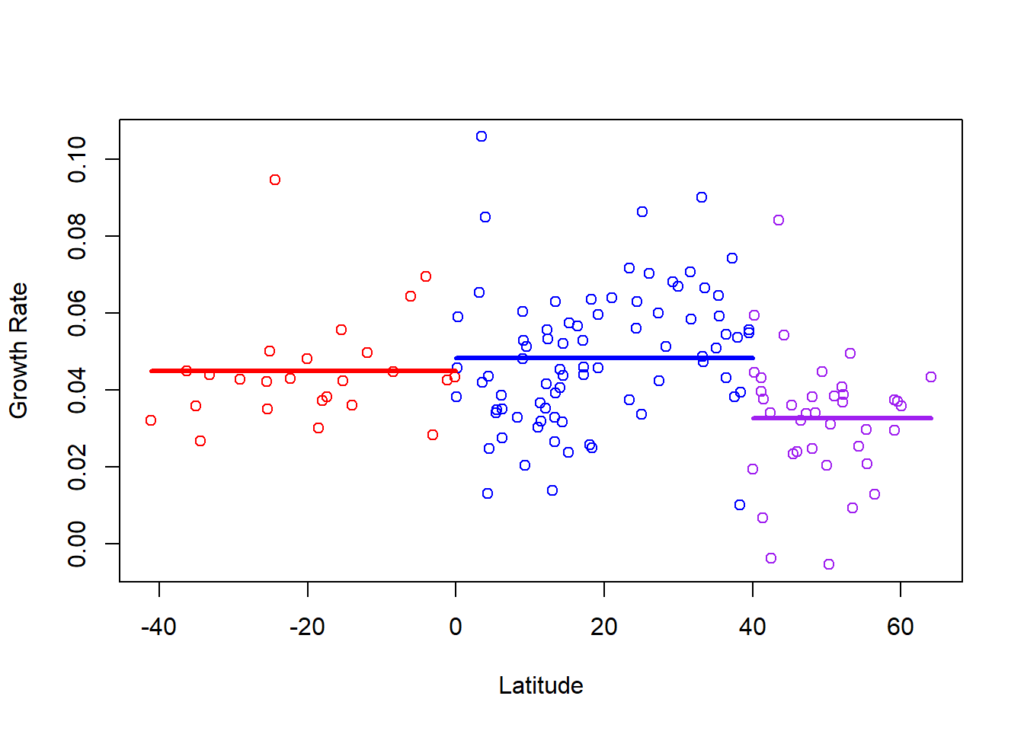
4.1.5 ANOVA of 3 Groups’ Growth Rates
# Add group labels to PWT
pwt_4 <- pwt_3
pwt_4[latitude<0, "group" := 1]
pwt_4[latitude>=0 & latitude<40, "group" := 2]
pwt_4[latitude>=40, "group" := 3]

anova_fit <- aov(growth_rate ~ as.factor(group), data = pwt_4)
# Summary of the analysis
summary(anova_fit)
## Df Sum Sq Mean Sq F value Pr(>F)
## as.factor(group) 2 0.23 0.11452 14.77 3.95e-07 ***
## Residuals 7865 60.98 0.00775
## ---
## Signif. codes: 0 '***' 0.001 '**' 0.01 '*' 0.05 '.' 0.1 ' ' 1
## 1924 observations deleted due to missingnessTukeyHSD(anova_fit)## Tukey multiple comparisons of means
## 95% family-wise confidence level
##
## Fit: aov(formula = growth_rate ~ as.factor(group), data = pwt_4)
##
## $`as.factor(group)`
## diff lwr upr p adj
## 2-1 0.003777896 -0.002306716 0.009862508 0.3126530
## 3-1 -0.009611521 -0.016798392 -0.002424650 0.0049084
## 3-2 -0.013389417 -0.019164059 -0.007614775 0.0000002There is indeed a significant difference in means for growth rates for group 3, while groups 1 and 2 do not appear to be different. Therefore, location appears to offer an explanation of growth, thus supporting Hall and Jones’ social infrastructure contention.
Causal analysis as performed in the previous section will be
ineffectual given the categorical nature of the location variable as
proxied by latitude against the panel data of the country’s growth.
4.1.6 Does This Hold Since 2000?
pwt_5 <- pwt_4[pwt_4$year >= 2000,]


pwt_5[, "growth_rate" := lapply(.SD, rate), by = country, .SDcols = "rgdpe"]
pwt_5[, "mean_growth_rate" := lapply(.SD, mean, na.rm = TRUE), by = country, .SDcols = "growth_rate"]

plot(pwt_5$latitude, pwt_5$mean_growth_rate, xlab="Latitude", ylab = "Growth Rate")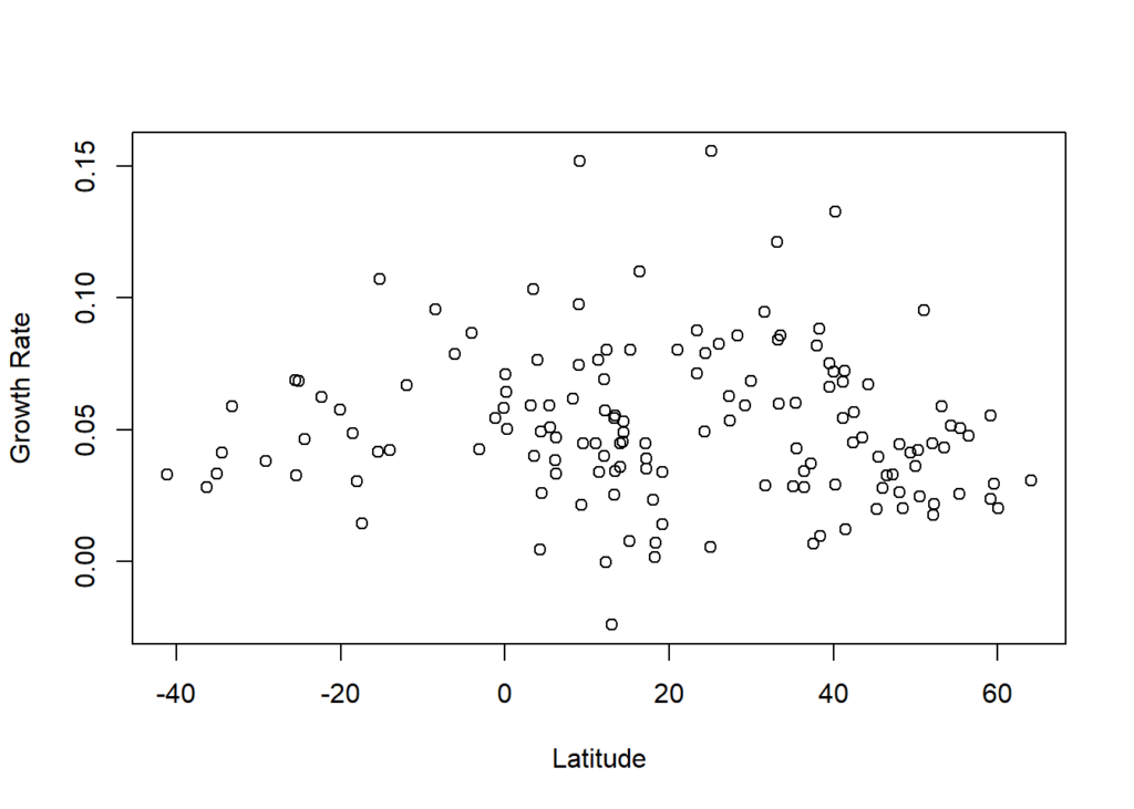
group_1_growth <- mean(pwt_5[latitude<0, ]$mean_growth_rate)
group_2_growth <- mean(pwt_5[latitude>=0 & latitude<40, ]$mean_growth_rate)
group_3_growth <- mean(pwt_5[latitude>=40, ]$mean_growth_rate)

plot(pwt_5$latitude, pwt_5$mean_growth_rate, xlab="Latitude", ylab = "Growth Rate",
     col = ifelse(pwt_5$latitude<0, 'red',
                  ifelse(pwt_5$latitude<40, 'blue', 'purple')))
segments(min(pwt_5$latitude), group_1_growth, 0, group_1_growth, col = 'red', lwd = 3)
segments(0, group_2_growth, 40, group_2_growth, col = 'blue', lwd = 3)
segments(40, group_3_growth, max(pwt_5$latitude), group_3_growth, col = 'purple', lwd = 3)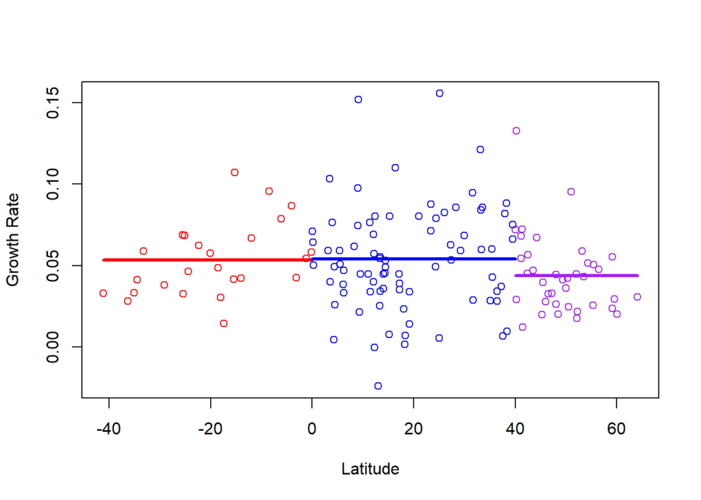
anova_fit <- aov(growth_rate ~ as.factor(group), data = pwt_5)
# Summary of the analysis
summary(anova_fit)
## Df Sum Sq Mean Sq F value Pr(>F)
## as.factor(group) 2 0.049 0.024345 3.811 0.0223 *
## Residuals 2445 15.621 0.006389
## ---
## Signif. codes: 0 '***' 0.001 '**' 0.01 '*' 0.05 '.' 0.1 ' ' 1
## 144 observations deleted due to missingnessTukeyHSD(anova_fit)## Tukey multiple comparisons of means
## 95% family-wise confidence level
##
## Fit: aov(formula = growth_rate ~ as.factor(group), data = pwt_5)
##
## $`as.factor(group)`
## diff lwr upr p adj
## 2-1 0.0005119148 -0.009889547 0.010913377 0.9926828
## 3-1 -0.0097188508 -0.021426305 0.001988603 0.1259507
## 3-2 -0.0102307656 -0.019169852 -0.001291679 0.0200266There is still significant difference in mean growth rates since 2000, and closer inspection via the Tukey test shows it is a negative difference in group 3, the northern countries.
4.1.7 Year by Year Average Growth Rates for Each Group
What if we examine the trajectory of the p-values in the difference between groups 3 and 2 year by year…
p_value <- numeric()

for(i in unique(pwt_4$year)){
  index <- which(i==unique(pwt_4$year))

  pwt_5 <- pwt_4[pwt_4$year >= i, ]
  pwt_5[, "mean_growth_rate" := lapply(.SD, mean, na.rm = TRUE), by = country,
        .SDcols = "growth_rate"]

  group_1_growth <- mean(pwt_5[latitude<0, ]$mean_growth_rate)
  group_2_growth <- mean(pwt_5[latitude>=0 & latitude<40, ]$mean_growth_rate)
  group_3_growth <- mean(pwt_5[latitude>=40, ]$mean_growth_rate)

  anova_fit <- aov(mean_growth_rate ~ as.factor(group), data = pwt_5)

  a <- TukeyHSD(anova_fit)
  p_value[index] <- a[[1]][3,4]
}

plot(head(unique(pwt_4$year), length(na.omit(p_value))), na.omit(p_value),
     xlab = "Year", ylab = "p-value group 3-2 Difference")
We fail to reject the differences in group means over the last 6 years (since 2011). Maybe this is the convergence they were speaking of…